부분최소제곱법(Partial Least Squares, PLS)
`부분최소제곱법(Partial Least Squares, PLS)`은 X의 선형결합의 분산을 최대화하는 것과 더불어 X의 선형결합 Z와 Y간의 공분산을 최대화하는 변수를 추출하는 방법이다.

PLS는 Y와의 공분산이 높은 k개의 선형조합 변수를 추출(Supervised feature extraction)하는 방식이다. PLS(부분최소제곱)의 용어는 선형조합으로 추출된 변수가 설명하지 못하는 부분에(데이터 일부분) 지속적으로 최소제곱법을 사용하는 것에서 유래했다. PLS의 주요 목적은 PCA와 동일하게 회귀 및 분류 모델을 구축하고, 데이터의 차원을 축소시키는 것이다. 그러나 PCA와의 차이점은 추출된 변수가 PCA에서는 반영하지 못했던 Y와의 상관관계를 반영한다는 점이다. 이러한 PLS를 통해 적은 수의 추출된 변수로 효율적인 모델의 구축이 가능하다.
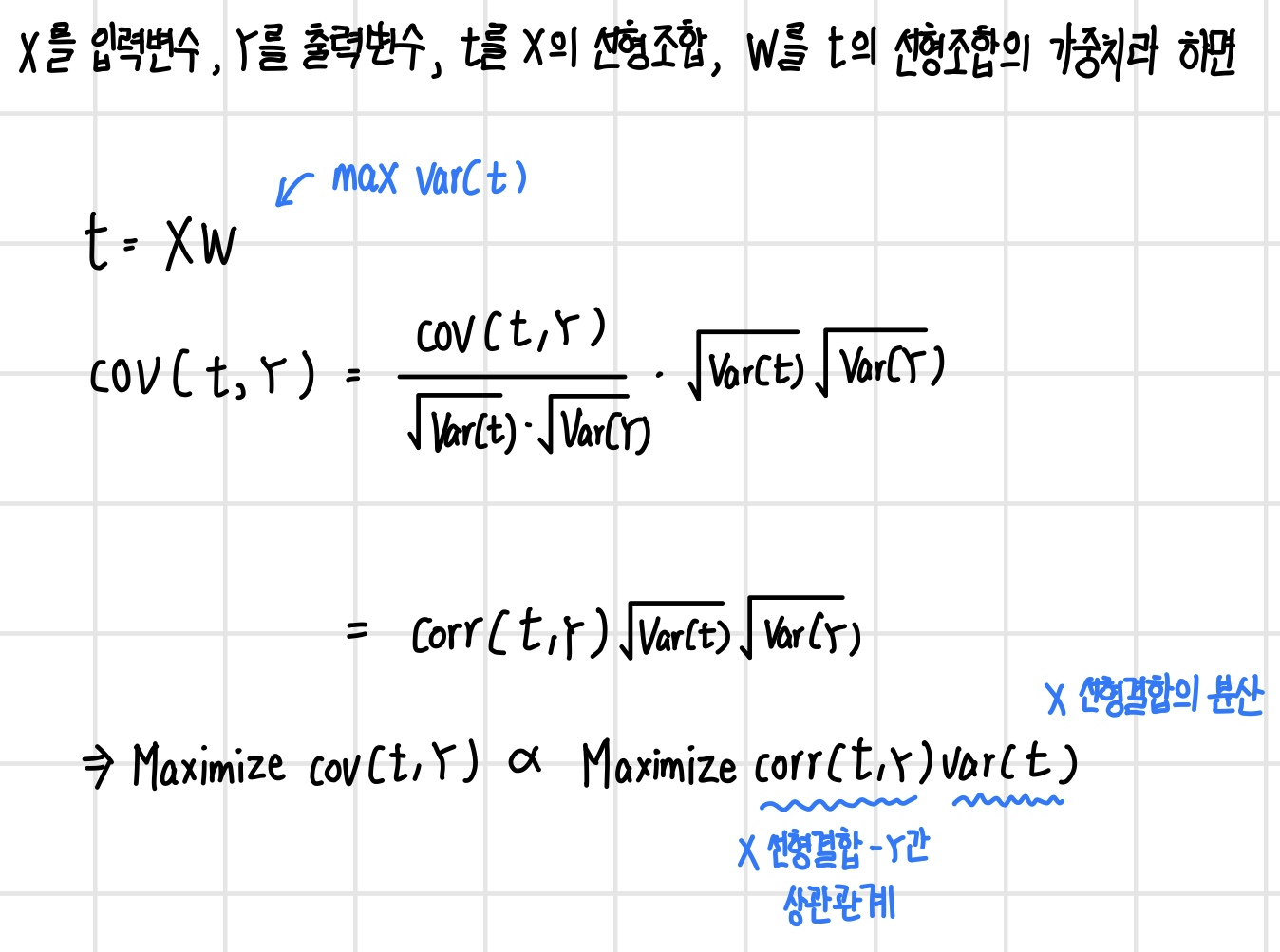
X를 입력변수, Y를 출력변수, t를 X의 선형조합, w를 선형조합의 가중치라 할 때, PLS component t는 w와 X의 선형결합으로 표현할 수 있다. PCA의 경우 이 t의 분산을 최대로 하지만 PLS는 추가적으로 t와 Y의 공분산 또한 최대화하는 것을 목표로 한다. t와 Y의 공분산을 계산하는 식에 약간의 트릭을 주면 다음과 같이 표현할 수 있으며, 결론적으로 t와 Y의 공분산을 최대화하는 것은 X와 w의 선형결합인 t의 분산을 최대화하는 것과 더불어 t와 Y의 correlation을 최대화하는 것으로 표현할 수 있다.
PLS - 변수 추출 방법
PLS Component t를 계산하는 것은 결국 가중치 w를 어떻게 설정하는가에서 시작된다. 이 w를 계산하는 방법은 다음과 같다.

NIPALS(Nonlinear Iterative Partial Least Squares) Algorithm
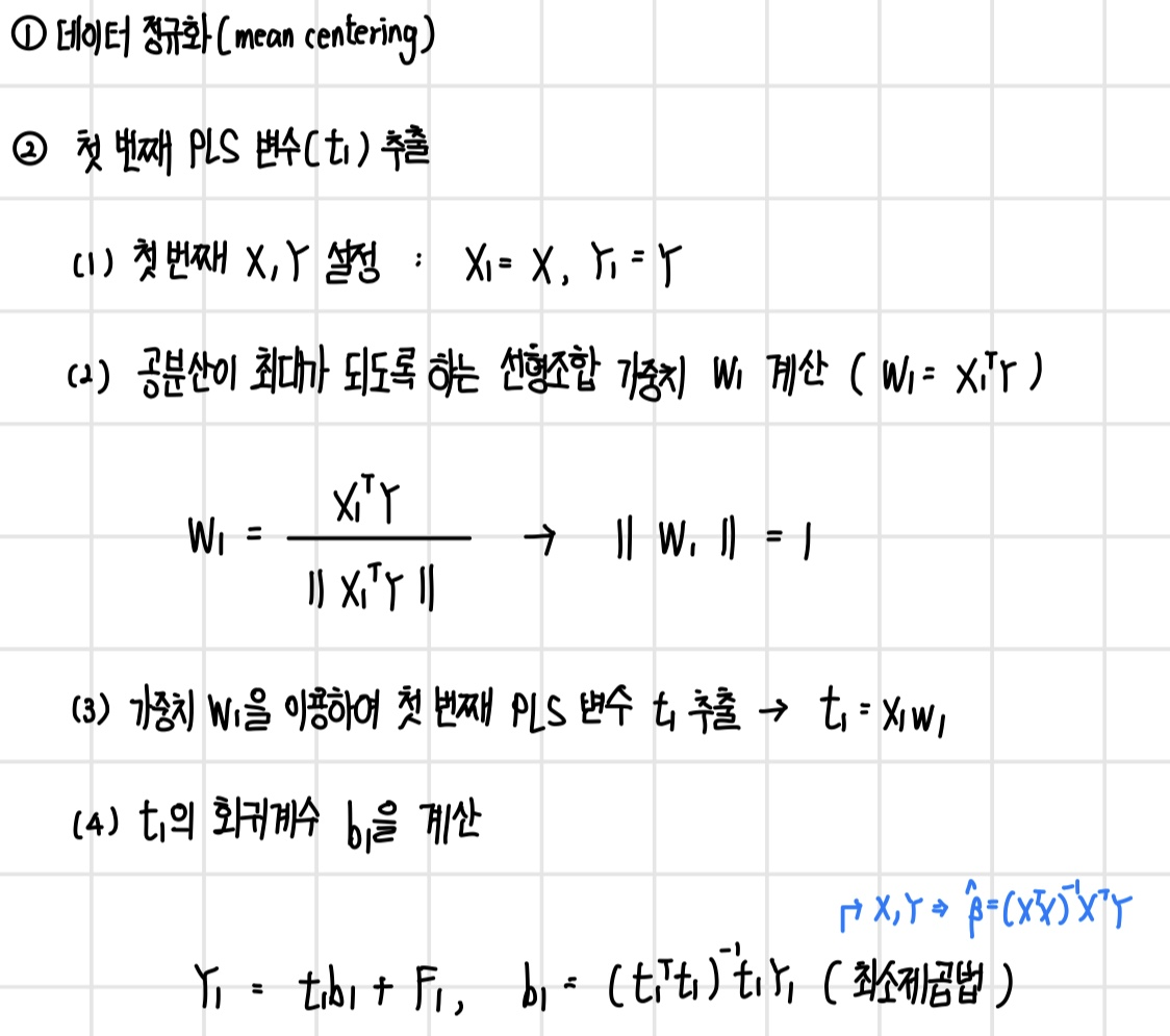
PLS Component t와 그에 대한 회귀 계수를 계산하는 방법은 다음과 같다. 먼저 데이터에 대한 데이터 정규화를 수행한 후, 첫 번째 PLS 변수(t1)를 추출한다.
이후 추출한 t1이 기존 X, Y에 대해 각각 설명하는 부분을 제외하고 잔차, 즉 t1이 설명하지 못하는 부분을 Y2와 X2로 설정하고 이에 대하여 또다서 두 번째 PLS 변수(t2)와 회귀계수 b2를 계산한다.

이렇게 같은 방식으로 원하는 k번째 PLS 변수까지 추출을 한다. 결국 계속 전체 데이터의 설명하지 못한 부분들(partial)에 대해서 최소 제곱법을 수행한다.

마지막으로 충분한 PLS 계수가 추출되었다면 앞서 계산한 PLS 변수와 회귀 계수들로 선형 회귀식을 통해 예측 값을 계산한다.

PLS - 추출 변수의 수 결정
PLS 변수를 추출하는 방법과 예측 값을 계산하는 방법은 알았지만, 결국 궁극적인 목표인 `차원 축소(dimension reduction)`은 아직 달성하지 못했다. 이를 위해선 추출변수의 수(Number of PLS components) k를 결정해야 한다. 이를 위해서 k를 순차적으로 증가시키며 예측 결과를 확인하고, 가장 좋은 예측 결과를 보이는 k를 선택하면 된다. 다음과 같은 예에선 k를 5로 설정한다.

이 포스팅은 고려대학교 산업경영공학부 김성범 교수님 유튜브 핵심 머신러닝 강의를 공부하고 작성한 글입니다.
(이미지 출처 - 핵심 머신러닝)